Using the seven-step SGD process for Fashion MNIST
I apply all the lessons we’ve learned so far on the Fashion MNIST dataset. This requires us learning a few new concepts like optimisers, ReLU, nonlinearity and so on.
In the previous post I used the seven-step process to fit to an unknown function. The process as a whole is fairly simple to get your head around, but there are a good few details to keep track of along the way. This will continue to be the case as we get into this walkthrough of how to do the same for the Fashion MNIST pullover vs dress data.
Getting our data into the right format
The first thing we need to handle is making sure our data is in the right format, shape and so on. We begin by downloading our data and splitting the data into training and test sets.
training_data = datasets.FashionMNIST( root="data", train=True, download=True, transform=ToTensor())test_data = datasets.FashionMNIST( root="data", train=False, download=True, transform=ToTensor())training_dresses = [item[0][0] for item in training_data if item[1] ==3]training_pullovers = [item[0][0] for item in training_data if item[1] ==2]test_dresses = [item[0][0] for item in test_data if item[1] ==3]test_pullovers = [item[0][0] for item in test_data if item[1] ==2]training_dresses_tensor = torch.stack(training_dresses)training_pullovers_tensor = torch.stack(training_pullovers)test_dresses_tensor = torch.stack(test_dresses)test_pullovers_tensor = torch.stack(test_pullovers)training_dresses_tensor.shape, test_dresses_tensor.shape
We transform our images tensors from matrices into vectors with all the values one after another. We create a train_y vector with our labels which we can use to check how well we did with our predictions.
We create datasets out of our tensors. This means that we can feed our data into our training functions in the way that is most convenient (i.e. an image is paired with the correct label).
As in the previous times where we’ve done this, we initialise our parameters or weights with random values. This means that for every pixel represented in the images, we’ll start off with purely random values. We initialise our bias to a random number as well.
# calculating a prediction for our first image(train_x[0]*weights.T).sum() + bias
tensor([2.8681], grad_fn=<AddBackward0>)
Matrix multiplication to calculate our predictions
We’ll need to make many calculations like the one we just made, and luckily the technique of matrix multiplication helps us with exactly the scenario we have: we want to multiply the values of our image (laid out in a single vector) with the weights and to add the bias.
In Python, matrix multiplication is carried out with a simple @ operator, so we can bring all of this together as a function:
Our accuracy is pretty poor! A lot worse than even 50/50 luck which is what you’d expect to get on average from a random set of initial weights. Apparently we had a bad draw of luck this time round!
A loss function to evaluate model performance
We now need a loss function which will tell us how well we are doing in our predictions, and that can be used as part of the gradient calculations to let us know (as we iterate) how to update our weights.
The problem, especially in the data set we’re working with, is that we have a binary probability: either it’s a dress or a pullover. Zero or one. Unlike in a regression problem, or something similar, we don’t have any smooth selection of contiguous values that get predicted. We have zero or one.
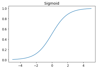
At this point we learn about the sigmoid function which is a way to reframe this problem in a way that we can use to our advantage. The sigmoid function when plotted looks like this:
This function, as you can see, takes any input value and squashes it down such that the output value is between 0 and 1. It also has a smooth curve, all headed in the same direction, between those values. This is ideal for our situation. The first thing we must do as part of our loss function, therefore, is to apply the sigmoid function to the inputs.
This torch.where(...) function is a handy way of iterating through all our data, checking whether our target is 1 or not, then outputting the distance from the correct prediction and calculating the mean of these predictions across the entire dataset.
DataLoaders and Datasets
We’ve already created datasets for our training and validation data. The process of iterating through our data, however, requires some thought as to how we’ll do it. Our options:
we could iterate through the entire dataset, making the relevant loss and gradient calculations and adjusting the weights but this might make the process quite long, even though we’d benefit from the increased accuracy this would bring since we’d be seeing the entire dataset each iteration.
we could do our calculations after just seeing a single image, but then our model would be over-influenced and perturbed by the fluctuations from image to image. This also wouldn’t be what we want.
In practice, we’ll need to choose something in between. This is where mini-batches or just ‘batches’ come in. These will be need to be large enough (and randomly populated!) that our model can meaningfully learn from them, but not so large that our process takes too long.
Luckily, we have the abstraction of the DataLoader which will create all our randomly assigned batches for us.
We had 91% accuracy on our validation dataset last time we tried this with pixel similarity.
After 30 epochs of training with our new process we’ve achieved 96%, but we could still do better! We’ll tackle that in the next post.
Optimising with an Optimiser
Everything that we’ve been doing so far is so common that there is pre-built functionality to handle all of the pieces.
our linear1 function (which calculated predictions based on our weights and biases) can be replaced with PyTorch’s nn.Linear module. Actually, nn.Linear does the same thing as our initialise_params and our linear1 function combined.
# initialises our weights and bias, and is our model / functionlinear_model = nn.Linear(28*28, 1)
Our PyTorch module carries an internal representation of our weights and our biases:
an optimiser bundles the step functionality and the zero_grad_ functionality. In the book we see how to create our own very basic optimiser, but fastai provides the basic SGD class which we can use that handles these same behaviours.
We’ll need to amend our training function a little to take this into account:
So there we have it. We learned how to create a linear learner. Obviously 96.8% accuracy is pretty good, but it could be better. Next time we’re going to add the final touches to this process by creating a neural network, adding layers of nonlinearity to ensure our function can fit the complex patterns in our data.